Medium - Data Scientists, The 5 Graph Algorithms that you should know
in Trend
Trend 파악을 Medium 기고문 요약 포스팅 - 데이터 과학자라면 당신이 꼭 알아야 할 5가지 그래프 알고리즘에 대해; 왜냐면 그래프 분석이 미래이기 때문입니다.

1.Connected Components

A graph with 3 connected components
Applications
Code

Graph with Some random distances
edgelist = [
['Mannheim', 'Frankfurt', 85], ['Mannheim', 'Karlsruhe', 80], ['Erfurt', 'Wurzburg', 186],
['Munchen', 'Numberg', 167], ['Munchen', 'Augsburg', 84], ['Munchen', 'Kassel', 502],
['Numberg', 'Stuttgart', 183], ['Numberg', 'Wurzburg', 103], ['Numberg', 'Munchen', 167],
['Stuttgart', 'Numberg', 183], ['Augsburg', 'Munchen', 84], ['Augsburg', 'Karlsruhe', 250],
['Kassel', 'Munchen', 502], ['Kassel', 'Frankfurt', 173], ['Frankfurt', 'Mannheim', 85],
['Frankfurt', 'Wurzburg',  217], ['Frankfurt', 'Kassel', 173], ['Wurzburg', 'Numberg', 103],
['Wurzburg', 'Erfurt', 186], ['Wurzburg', 'Frankfurt', 217], ['Karlsruhe', 'Mannheim', 80],
['Karlsruhe', 'Augsburg', 250], ["Mumbai","Delhi",400],["Delhi","Kolkata",500],
["Kolkata", "Bangalore",600],["TX", "NY",1200],["ALB", "NY",800]
]
g = nx.Graph()
for edge in edgelist:
    g.add_edge(edge[0],edge[1], weight = edge[2])
for i, x in enumerate(nx.connected_components(g)):
    print("cc"+str(i)+":",x)
------------------------------------------------------------
cc0: {'Frankfurt', 'Kassel', 'Munchen', 'Numberg', 'Erfurt', 'Stuttgart', 'Karlsruhe', 'Wurzburg', 'Mannheim', 'Augsburg'}
cc1: {'Kolkata', 'Bangalore', 'Mumbai', 'Delhi'}
cc2: {'ALB', 'NY', 'TX'}
2.Shortest Path
Applications


Code
print(nx.shortest_path(g, 'Stuttgart','Frankfurt',weight='weight'))
print(nx.shortest_path_length(g, 'Stuttgart','Frankfurt',weight='weight'))
--------------------------------------------------------
['Stuttgart', 'Numberg', 'Wurzburg', 'Frankfurt']
503
for x in nx.all_pairs_dijkstra_path(g,weight='weight'):
    print(x)
--------------------------------------------------------
('Mannheim', {'Mannheim': ['Mannheim'],
'Frankfurt': ['Mannheim', 'Frankfurt'],
'Karlsruhe': ['Mannheim', 'Karlsruhe'],
'Augsburg': ['Mannheim', 'Karlsruhe', 'Augsburg'],
'Kassel': ['Mannheim', 'Frankfurt', 'Kassel'],
'Wurzburg': ['Mannheim', 'Frankfurt', 'Wurzburg'],
'Munchen': ['Mannheim', 'Karlsruhe', 'Augsburg', 'Munchen'],
'Erfurt': ['Mannheim', 'Frankfurt', 'Wurzburg', 'Erfurt'],
'Numberg': ['Mannheim', 'Frankfurt', 'Wurzburg', 'Numberg'],
'Stuttgart': ['Mannheim', 'Frankfurt', 'Wurzburg', 'Numberg', 'Stuttgart']})
('Frankfurt', {'Frankfurt': ['Frankfurt'],
'Mannheim': ['Frankfurt', 'Mannheim'],
'Kassel': ['Frankfurt', 'Kassel'],
'Wurzburg': ['Frankfurt', 'Wurzburg'],
'Karlsruhe': ['Frankfurt', 'Mannheim', 'Karlsruhe'],
'Augsburg': ['Frankfurt', 'Mannheim', 'Karlsruhe', 'Augsburg'],
'Munchen': ['Frankfurt', 'Wurzburg', 'Numberg', 'Munchen'],
'Erfurt': ['Frankfurt', 'Wurzburg', 'Erfurt'],
'Numberg': ['Frankfurt', 'Wurzburg', 'Numberg'],
'Stuttgart': ['Frankfurt', 'Wurzburg', 'Numberg', 'Stuttgart']})
....
3.Minimum Spanning Tree
An Undirected Graph and its MST on the right.
Applications
Code
# nx.minimum_spanning_tree(g) returns a instance of type graph
nx.draw_networkx(nx.minimum_spanning_tree(g))
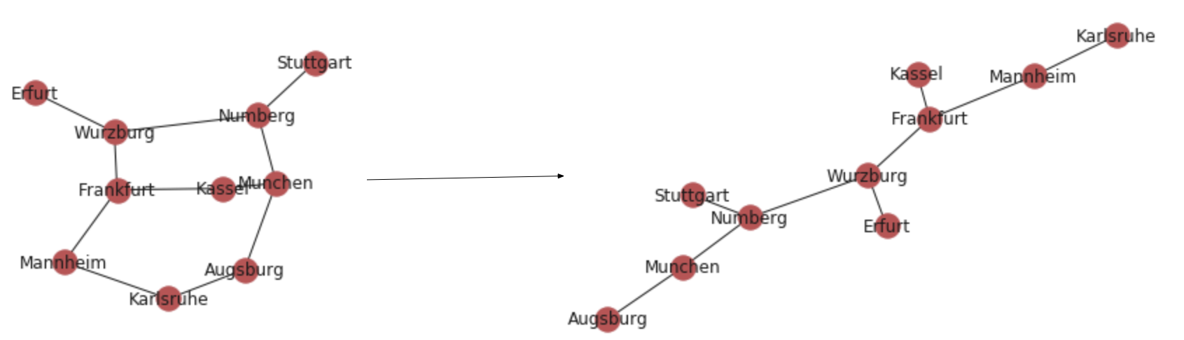
The MST of our graph.
4.Pagerank

Applications
Code
# reading the dataset
fb = nx.read_edgelist('../input/facebook-combined.txt', create_using = nx.Graph(), nodetype = int)
pos = nx.spring_layout(fb)
import warnings
warnings.filterwarnings('ignore')
plt.style.use('fivethirtyeight')
plt.rcParams['figure.figsize'] = (20, 15)
plt.axis('off')
nx.draw_networkx(fb, pos, with_labels = False, node_size = 35)
plt.show()

FB User Graph
pageranks = nx.pagerank(fb)
print(pageranks)
------------------------------------------------------
{0: 0.006289602618466542,
 1: 0.00023590202311540972,
 2: 0.00020310565091694562,
 3: 0.00022552359869430617,
 4: 0.00023849264701222462,
........}
import operator
sorted_pagerank = sorted(pagerank.items(), key=operator.itemgetter(1),reverse = True)
print(sorted_pagerank)
------------------------------------------------------
[(3437, 0.007614586844749603), (107, 0.006936420955866114), (1684, 0.0063671621383068295),
(0, 0.006289602618466542), (1912, 0.0038769716008844974), (348, 0.0023480969727805783),
(686, 0.0022193592598000193), (3980, 0.002170323579009993), (414, 0.0018002990470702262),
(698, 0.0013171153138368807), (483, 0.0012974283300616082), (3830, 0.0011844348977671688),
(376, 0.0009014073664792464), (2047, 0.000841029154597401), (56, 0.0008039024292749443),
(25, 0.000800412660519768), (828, 0.0007886905420662135), (322, 0.0007867992190291396),......]
first_degree_connected_nodes = list(fb.neighbors(3437))
second_degree_connected_nodes = []
for x in first_degree_connected_nodes:
    second_degree_connected_nodes+=list(fb.neighbors(x))
second_degree_connected_nodes.remove(3437)
second_degree_connected_nodes = list(set(second_degree_connected_nodes))
subgraph_3437 = nx.subgraph(fb,first_degree_connected_nodes+second_degree_connected_nodes)
pos = nx.spring_layout(subgraph_3437)
node_color = ['yellow' if v == 3437 else 'red' for v in subgraph_3437]
node_size =  [1000 if v == 3437 else 35 for v in subgraph_3437]
plt.style.use('fivethirtyeight')
plt.rcParams['figure.figsize'] = (20, 15)
plt.axis('off')
nx.draw_networkx(subgraph_3437, pos, with_labels = False, node_color=node_color,node_size=node_size )
plt.show()
Our most influential user(Yellow)
5.Centrality Measures
Applications
Code
pos = nx.spring_layout(subgraph_3437)
betweennessCentrality = nx.betweenness_centrality(subgraph_3437,normalized=True, endpoints=True)
node_size =  [v * 10000 for v in betweennessCentrality.values()]
plt.figure(figsize=(20,20))
nx.draw_networkx(subgraph_3437, pos=pos, with_labels=False,
                 node_size=node_size )
plt.axis('off')
